Hello! My name is Ethan, I'm a software engineer from California! This website was created out of my vast collection of photographs that I captured
throughtout the years and my deep passion for coding. I hope you find my work inspiring and
enjoyable. Thank you for visiting and have a wonderful day!! :)
I am an amateur photographer and software developer. 95% of all the pictures you will see
were taken by me. I also take pride in coding this website from scratch and validating
its standard with W3C. You have my every permission to use any content you see fit.
Words of Wisdom: It is important to be happy so please give your friends your smile when
they are not wearing one, just like me to the statue...
This is my most recent layout design. I added a fixed background, a photography and blog
panel, transition effect, and new dynamic features. A new page for Coding has been
created! In here I showcase a number of my programming projects that I worked on.
Please note that I purposely configurate a few fixed settings, so to maximize the user
experience, please go full-screen by hitting F11
Photography page no longer exists. Instead, I created a panel to opt three different
albums for ease of navigation. The presentation of galleries is a lot more organized and
sliders are compressed into one page.
Photos from Southeast Asia trip (Thailand, Cambodia, Malaysia) in 2018 are posted under
the Travel Album.
Portfolio This is my main gallery where I share
some of my favorite pictures!
Travel Album I'm blessed to capture so many great
memories in photos. This is my collection of all the countries I visited!
Other Project Here you can view my miscellaneous
work such as HDR, portraits, photo manipulation and many more!
Did you know that in Singapore, you are guilty until proven innocent? Or that
some beer are cheaper than water in Germany? What about the fact that there are more sheep than
people in New Zealand? Isn't it interesting that base on the Italian nationality law, jus
sanguinis, you have an Italian citizenship if one or both of your parents are citizens
of the nation regardless of your place of birth? In America, the thumb up is a congratulatory
expression but in the Arab world it is considered offensive (essentially, the middle finger).
Want to know more on my travels? Just click on the flags below to read about my adventure!
At the Rooftop of the World Sept 2017
You know the feeling of a hangover after a long night of drinks? Yeah it's like that except
it doesn't go away!! I was constantly tired, dizzy, lightheaded, and nauseous. I think my
altitude sickness at some point caused my attitude sickness. To order to enter Tibet you
have to have a special permit alongside with your Chinese visa.
One Megacity June 2013
The next day, with our Toyota Yaris, we drove to Downtown Toronto to enjoy the hustling and
bustling the city had to offer. Toronto earned the title of "Ethan's Best Architecture City"
because of its super modern glass use in office and residential buildings. Last year one of
my kids told me about Toronto and how beautiful its architecture was, but upon seeing it so
myself I must concur with her. There's a famous market called "St's Lawrence" which has all
sort of food including...
America, Land of Freedom and Opportunity June 2013
Chicago was the last destination on my trip. This
city is so beautiful, especially the architecture, after all this was where the Modern Architecture movement
started. It enjoys the attention of housing many of the world's tallest buildings including the Willis Tower
and Hancock Tower. Everyone here called me "Sir!" The weather was not necessarily hot, but super humid. I
stayed at the best hostel ever, located in the heart of Dowtown!
Visiting the Ghetto and Exploring Warsaw November 2011
The next day we were on a pirate ship to Gdynia and learned the history of Westerplatte, the
site that WWII “officially” began with German attack on Polish military installations. The
Germans opened fire first and killed 15 Polish soldiers but the Polish retaliated and killed
around a hundred Nazis. The following day we went to the Malbork Castle...
The Magical Kingdom of Beer and Wurst October 2011
On my first day here, I went to a bunch of squares and the Deutsches Musuem, which is a
museum of technology and science, the biggest of its kind in the world. This place surely
lives up to its name, I was there for over 5 hours and did finish. Coming here was like any
nerd’s dream and made me feel really proud to be an engineer...
Learning the city of Art and Music October 2011
In Vienna, I went to a residential house called “Hunderwasserhaus” which literally means
hundred water house. Hunderwasser is the name of the famous architect whose philosophy
opposed straight lines and simple color in modern architecture. It sounds weird to go to a
house in a foreign country but Hunderwasserhaus is actually one of the main attractions in
Vienna...
Exploring the Bohemian Empire October 2011
Prague in general is a very touristy, so taking a good picture is difficult. I often time had
to smell people’s armpit in the subway because it was simply too crowded. I also went to the
Dancing House, a famous architecture in league of the Sydney Opera House and other famous
buildings. As a structural engineer, I LOVED this building...
Delicious Food, Awesome Technology, Wealthy Nation, It's Singapore!
September 2010
I thought my life was complete after seeing the Sydney Opera House--then came the Esplanade
in Singapore. The Esplanade is the Singaporean version of the Sydney Opera House, and this
performing arts venue looks like a durian, an exotic fruit from Southeast Asia. The Youth
Olympics also took place when I was in Singapore...
Bridge and House of the Engineer August 2010
Henry Miller once said that “one’s destination is never a place, but a new way of seeing
things.” I, too, agree with this, in the sense that traveling and being exposed to other
cultures opens your eyes to a whole new dimension. There is so much that the world has to
offer and it's really up to us to...
One Big Chinatown Summer 2010
My hostel was in Tsim Sha Tsui along Nathan Road, a really long street popular for shopping
and food. It rained a lot on my first three days and there was a typhoon warning, but
overall the weather was really nice. My stay at the Chungking hostel was an experience
because I totally...
Fusion of European and Asian Influence Summer 2010
The main attraction (and most famous landmark) in Macau, besides all the casinos, is the San
Paulo Cathedral (enlisted as part of the UNESCO World Heritage Site Historic Centre). In the
late 16th century, the cathedral was one of the largest Catholic churches in Asia. However,
in early 19th century, a fire burned literally the whole church...
Internship and Adventure in New Zealand! July 2010
On the night of June 20, 2010 I knew my life wasn't going to be the same for a few months. I
knew that something tickled my twinkle and I couldn’t rest. The following day, I embarked on
a brand-new journey to find myself lost in a beautiful country, New Zealand, and furthermore
a sight-seeing city, Auckland. When I went through customs...
Journey to Rome with Me! Summer 2008
When I was a freshman in college, I had an opportunity to study abroad in Rome, Italy.
Spending five weeks in Rome that summer was one of the smartest things I ever did in my
young life. I met 15 exceptional and friendly students who all had the urge to learn with a
keen sense of curiosity...
According to Wikipedia, computer vision is an interdisciplinary field that deals with how
computers can be made for gaining high-level understanding from digital images or
videos. Computer vision tasks include methods for acquiring, processing, analyzing and
understanding digital images, and extraction of high-dimensional data from the real
world in order to produce numerical or symbolic information. It involves the development
of a theoretical and algorithmic basis to achieve automatic visual understanding. As a
scientific discipline, computer vision is concerned with the theory behind artificial
systems that extract information from images. The image data can take many forms, such
as video sequences, views from multiple cameras. In my graduate studies at Carnegie
Mellon University, I took a course in computer vision, which is my favorite course of
all time as well as the most difficult! These are projects I completed that will
encapsulate the basic idea of this powerful computer science concept. Please note
that I cannot provide my source code because these assignments may be reused in the
course.
Tracking
The first groundbreaking work on template tracking was the Lucas-Kanade tracker. It
basically assumes that the template undergoes constant motion in a small region. The
Lucas-Kanade Tracker works on two frames at a time, and does not assume any statistical
motion model throughout the sequence. The algorithm estimates the deformations between
two image frames under the assumption that the intensity of the objects has not changed
significantly betweenthe two frames. Starting with a rectangle $R_t$ on frame $I_t$, the
Lucas-Kanade Tracker aims to move it by an offset (u; v) to obtain another rectangle
$R_{t+1}$ on frame $I_{t+1}$, so that the pixel squared difference in the two rectangles
is minimized. According to Wikipedia, $A^TA$ is the structure tensor of the image at all
points in the rectangle. It's a gradient matrix that summarizes the principal directions
in a specified neighborhood of that point.
As for the conditions, $A^TA$ should be invertible, well-conditioned and should
not be too small due to noise (meaning the eigenvalues should not be too small).
Below is a tracking example of a car with little variations. This is totally
awesome because I always see bank robberies and car pursuit on T.V sky cams and
now I got to learn the technology and science behind it!
The above video is quite simple but real data is often corrupted by unknown image
noise or under varying illumination conditions. One way to address issue of
appearance variation is to use the principal component analysis.
$$I_{t+1}=I_t+\sum_{c=1}^k w_cB_c$$ The idea to optimize $w$ is to find the minimum
residual of the squared difference in the two rectangles. Suppose the residual is
$I_{t+1}(x+u,y+v)-I_t(x,y)$, it guarantees an optimized $w$ from above equation
provided that the residual is within an acceptable tolerance.
$$I_{t+1}(x+u,y+v)-I_t(x,y)=\sum_{c=1}^k w_cB_c \rightarrow r= \left[
\begin{array}{cccc} b_1 \; b_2 \cdots b_k \end{array} \right] \left[
\begin{array}{c} w_1 \\ w_2 \\ \vdots \\ w_k \end{array} \right] =bw \rightarrow
w=b^{-1}r $$
As you can see, this example isn't so perfect because of the variation in
appearance such as shading and lighting. Can you think of a way to make it
"easier" for computers to track these objects? How about reducing the color
channels by converting the frames to grayscale? Or use various empirical affine
motion equations to form a linear combination of bases.
Spatial Pyramid Matching for Scene Classification
The question of interest for this topic is "Given an image, can a computer
program determine where it was taken?" I used the Bag-of-Words (BoW) approach.
The BoW essentially trains the computer to reprense the world with visual words.
The idea is to give the computer many(!) data (images) to understand and
recognize so that it is "smart" enough to identify the next datum. This is where
data science like Machine Learning and Data Mining come to play to supervise the
dataset. To help the computer interpret the data, we filter the images and
extract their properties. A filter bank is a series of flters that captures
different visual properties. The Gaussian blurs are to smooth out the details by
reducing noise. For example, convolving with the Laplacian Gaussian kernel
allows easier detection of edges. Furthermore, the derivative of the Gaussian on
the x-direction detects a change in intensity along that axis, thus vertical
edges are more prominent. The same can be said for gradient of the Gaussian in
respect to the y-axis which shows details on the horizontal edges. Bag of words
is simple and efficient, but it discards information about the spatial structure
of the image and this information is often valuable. One way to alleviate this
issue is to use spatial pyramid matching. The general idea is to divide the
image into a small number of cells, and concatenate the histogram of each of
these cells to the histogram of the original image, with a suitable weight. The
following outlines the basic idea of the algorithm.
Create a filter bank with different sort of scales, orientations, and
bandwidths to measure the responses of the images.
Randomly select a number of pixels to examine and group these pixels'
response in a cluster. From these data we are able to compile a dictionary
of visual words.
Run through all images and obtain the visual word with the minimum distance
on each pixel. Extract the frequency histogram where the number of bins is
the number of words. For a more accurate result, use Spatial Pyramid
Matching
Find the instance word with the largest similarity and assign its category
to the image.
Keypoints - Detectors, Descriptors and Matching
Interest point detectors find particularly salient points in an image upon which
we can extract a feature descriptor. In our case, we will be using BRIEF. Once
we have extracted the interest points, we can use descriptors to match them
between images to do neat things like panorama stitching or scene
reconstruction. Keypoints are found by using the Difference of Gaussian (DoG)
detector. This detector finds points that are extrema in both scale and space of
a DoG pyramid. The objective of this assignment was to learn a tomato soup can
and be able to recognize and match it from various angles. We accomplish this by
identifying points of interest and match them with a descriptor. One simple
descriptor is BRIEF which uses the Hamming distance to compute the similarity
between the potential matches. The belowed image on the left shows the ideals
points of critical contrast that I needed to match and my results on the right
image.
Unfortunately, my algorithm does not yield any correct
matches. The closest and best result I obtained was the top left. Of course, if
the test image compares to itself, the percentage of correct matches would be
100%, however I believe once rotated, the derivative of Gaussian is more
difficult in terms of computing the gradient at the edges. In other words, the
eigenvalues is distorted due to the change of orientation.
Homographies
Robots often deal with planes, whether in the form of walls, ground, or some
other at surface. When two cameras observe a plane, there exists a relationship
between the images captured. This relationship is defined by a 3x3
transformation matrix, called a planar homography. This was definitely one of my
more favorite topics to learn in Computer Vision because it is highly practical.
Let's suppose a robot is at war, it needs to be able to "stitch" the planar
images that it "sees" to interpret it as a warzone and take action. A planar
homopgrahy allows us to compute how a planar scene would look from a second
camera location give only the first image! Furthermore, we can extrapolate any
camera angle from any location without knowing any internal camera parameters.
Can you quess what simple use of homography? Panoramas! For this assignment, I
was given two images of the Taj Mahal and I had to use homographies to create a
panorama image of the same scene.
Suppose $p \propto Hq$ where
$p=[x',y',z']^T$ and $q=[x,y,z]^T$ for $p,q$ respectively, then $$ \left \{
\begin{array}{c} x'\\y'\\z' \end{array} \right\} \sim \left[ \begin{array}{ccc}
h_{11} & h_{12} & h_{13} \\ h_{21} & h_{22} & h_{23} \\ h_{31} & h_{32} & h_{33}
\end{array} \right] \left \{ \begin{array}{c} x\\y\\z \end{array} \right\}
\rightarrow \left \{ \begin{array}{c}
x'=\frac{h_{11}x+h_{12}y+h_{13}}{h_{31}x+h_{32}y+h_{33}}\\\\y'=\frac{h_{21}x+h_{22}y+h_{23}}{h_{31}x+h_{32}y+h_{33}}
\end{array} \right. $$\\ If we multiply both sides by the denominator and arrange,
we get $$ \left \{ \begin{array}{c} x'=h_{11}x+h_{12}y+h_{13}-h_{31}xx'-h_{32}yx'-x'
\\ y'=h_{21}x+h_{22}y+h_{23}-h_{31}xy'-h_{32}yy'-y' \end{array} \right. $$ To
minimize the homogenous linear least squares system we seek $arg \; min ||Ah|| = arg
\; min \;h^TA^TAh = \lambda_{min}$ If we decompose A using SVD method, the planar
homography is precisely the last column of D corresponding to the smallest
eigenvalue. Furthermore, if the eigenvalues are zero, h is exactly determined and
fits all the points perfect. If the values are positive, the system is
overdetermined and a residual will exist.
I designed and built a simple software package/interface for finite element analysis. The
main idea of this project was to provide students access to analytical studies of the
finite element method. Students should be able to obtain a basic understanding of the
importance of FEM and how it works at the elementary level. Note that some calculus
(including linear algebra and differential equations) is required to understand the
mathematics.
Click on the icon to download the graphical user interface.
Click on the
icon to download the lesson PDF.
Linear & Quadratic Interpolation of Continuous
Function
§ Methods of Weighted Residual to Obtain Governing Weak Form
Consider:
$-(k\hat{u}')'+b\hat{u}'+c\hat{u}=f$ Residual:
$r(\hat{u})=-(k\hat{u}')'+b\hat{u}'+c\hat{u}-f$ Multiply by test function v such
that v and u are in the same space (thus v also satisfies EBC) and integrate over
domain: $$\int_0^L r(\hat{u})vdx = 0 \rightarrow \int_0^L
[-(k\hat{u}')'+b\hat{u}'+c\hat{u}-f]vdx=0 $$ Suppose v is sufficiently smooth so that we
can integrate the 1st term by parts: $$\int_0^L -(k\hat{u}')'vdx=-(k\hat{u}')v|^L_0 +
\int_0^Lk\hat{u}'v'dx$$ Suppose the initial boundary is zero, then u(0)=0, it follows
that that v at x=0 must also be 0 and we have $$\int_0^L k\hat{u}'v'dx +
\int_0^Lc\hat{u}vdx - \int_0^Lfvdx - T_vv(L)=0$$
§ Numerical Approximation: Galerkin Method in Weak Form
Let $\hat{u} \sim u_N =
\sum_{k=1}^N \alpha_k \phi_k(x)$, then $\hat{u} \sim u_N = \sum_{i=1}^N \beta_i
\phi_i(x)$ $$\int_0^L k \left( \sum_{k=1}^N \alpha_k \phi_k'(x) \right)\left(
\sum_{i=1}^N \beta_i \phi_i'(x) \right)dx + \int_0^L c \left( \sum_{k=1}^N \alpha_k
\phi_k(x) \right)\left( \sum_{i=1}^N \beta_i \phi_i(x) \right)dx - \int_0^L f \left(
\sum_{i=1}^N \beta_i \phi_i(x) \right)dx-T_v \left( \sum_{i=1}^N \beta_i \phi_i(L)
\right)dx$$ Let $$K_{kj}=\int_0^L k(x)\phi_j'(x)\phi_k'(x)dx=K_{jk}$$
$$C_{kj}=\int_0^Lc(x)\phi_j(x)\phi_k(x)dx$$ $$f_k=\int_0^L f\phi_k(x)dx+\phi_k(L)$$ The
final equation to solve for is $$\sum_i B_i \left\{ \sum_k (K_{jk}+C_{jk})a_k -f_i
\right\}=0 \rightarrow \left\{ \sum_k (K_{jk}+C_{jk})a_k -f_i \right\}=0 \forall B_i,
\quad i=1, \dotsc ,n$$ The goal is to solve for $\alpha_k$ in $D\alpha=f$ where
$D_{jk}=K_{jk}+C_{jk}$
§ Selecting Appropriate Basic Functions
Consider the following linear basis
functions Trial functions:
$U_n(x)=\sum_{i=1}^n \alpha_i \phi_i(x)$ Test functions: $V_n(x)=\sum_{i=1}^n
\beta_i X_i(x)$ How do we choose a $\phi(x)$ such that $\hat{u}$ satisfies the
boundary conditions?
Approximated solution using quadratic basic function converges to the analytical
solution quicker than linear functions.
We generally work with the weak form to minimize the residual
The smaller the mesh, the more accurate $u(x,\phi)$ will be
In the discussion of error analysis, quadratic algorithm yields a smaller error
than linear due to a larger big O.
Torsional Analysis of Solid Elliptical Membrane
Suppose we have the schematic diagram below and the assoicated nodes.
We first note the symmetry of the membrane and simplify the model by considering only
the first quadrant. Equation of Ellipse is $$(\frac{x}{a})^2+(\frac{y}{b})^2=1$$ We
segment each of the quadrant into two individual meshes: Biquadratic Quadralateral
and Bilinear Triangle Rectangular Element: $Nodes [1 \;2 \;3 \;5 \;6 \;7 \;8 \;9
\;0]$ Triangular Element: $Nodes [3 \;4 \;12 \;11 \;10 \;7]$
§ Procedure
The following demonstrates the procedure in calculating the
stiffness matrix and loading vector of the elements. 1Choose $\Omega$ and $\Phi_j$, $j=1,2,...,N_e$ and specify the x-y
coordinates $(x_1,y_1),(x_2,y_2),...,(x_N,y_N)$ of nodal points of each
element. 2Specify a set of $N_i$ integration points $(\xi_l,\eta_l), \;
l=1,2,...,N_l$ and quadrature weights for $\Omega$} 3Calculate the values of $\Phi_j, \partial \Phi_j / \partial \xi,
\partial \Phi_j / \partial \eta$ at the integration points.} 4Calculate the values of $x=x(\xi,\eta), y=y(\xi,\eta)$ and their
derivatives at the integration points.} 5Calculate the values of the Jacobian and the functions $\partial \xi
/\partial x, \partial \xi / \partial y, \partial \eta / \partial x, \partial
\eta / \partial y$} 6Compute $\partial \phi_j^e / \partial x$ and $\partial \phi_j^e /
\partial y$} 7Calculate the values of $k, b$ and $f$
We may skip this step if we assume $k=f=1$ 8Using the results of steps 3 to 7, calculate the values of the
integrands at the integration points and multiply each by
$w_i|\mathbf{J}(\xi_l,\eta_l)|$ 9Sum the numbers to obtain $k_{ij}^e$ and $f_i^e$
§ Numerical Integration
For the integration, we use numerical method to
determine the weights of the Gaussian Quadrature. $$\int_{-1}^1
f(x)dx=\sum_{i=1}^nw_if(t_i)$$ $$(n+1)L_{n+1}(t)-(2n+1)tL_n(t)+nL_{n-1}(t)=0, L_0(t)=1,
L_1(t)=t$$ $$ L_{n+1}(t)=\frac{(2n+1)tL_n(t)-nL_{n-1}(t)}{n+1} $$ For all n values
between 2 and 7, we have the following table
Graphical representation of the polynomials are below. Note that the x-intercepts
are the roots of $L_n(t)$ over n. Suppose $f(t)=t^k$
where $k=0,1,\ldots n$ $$\int_{-1}^1 f(t)dt = \int_{-1}^1 t^kdt =
\frac{1-(-1)^{k+1}}{k+1} = \sum_{i=1}^n w_if(t_i)$$ Thus the integration weights can
be determined by \begin{align}w_1t_1^k+\dots+w_nt_n^k=0 \qquad for \;
k=1,3,\dots,2n-1\\ w_1t_1^k+\dots+w_nt_n^k=\frac{2}{k+1} \qquad for \;
k=0,2,\dots,2n-2\end{align}
§ Torsional Properties
Physical quantities of interest, such as shear stresses
and the relationship between the twisting moment, or torque, T, and the angle of twist
$\theta$, per unit length of the shaft, can be determined as follows, once the potential
function u is known. $$T =2G\theta \int_\Omega ud\Omega$$ The shear stresses on the
elliptical cross-section are given by the following expressions: $$\sigma_{xz}=2G\theta
\frac{\partial u}{\partial y}, \; \sigma_{yz}=-2G\theta \frac{\partial u}{\partial x}$$
The stress function may be written as
$$\phi=B\lbrace(\frac{x}{a})^2+(\frac{y}{b})^2-1)\rbrace$$ But since $$\frac{\partial^2
\phi}{\partial x^2}+\frac{\partial^2 \phi}{\partial y^2}=-2G\theta$$ We get that
$$B=-\frac{a^2b^2G\theta}{a^2+b^2}$$ $$ \sigma_{xz}=\frac{\partial \phi}{\partial
y}=\frac{2By}{b^2}\quad \sigma_{yz}=-\frac{\partial \phi}{\partial x}=-\frac{2Bx}{a^2}
$$ $$ T =2G\theta \int_\Omega ud\Omega=-\pi B ab $$ We can also verfiy that
$$\phi=B\lbrace(\frac{x}{a})^2+(\frac{y}{b})^2-1)\rbrace=\phi=-\frac{a^2b^2G\theta}{a^2+b^2}\lbrace(\frac{x}{a})^2+(\frac{y}{b})^2-1)\rbrace$$
With $u_h^e$ from part (i), multiply this with $\Phi_j$ for quadrilateral and
triangular elements from page 198 and 204, respectively. You could ignore the
nodes on boundary since it will be zero. For simplicity, consider working with
one quadrant.
Use numerical integration to compute the integral similar to step 8 from part
(i)
Repeat Steps 1 and 2 for the other element.
Sum everything from both elements.
Assume G and $\theta$ to be 1, multiply result from step (4) by 8 (2 from the
constant term of the equation, and 4 since we have four quadrants.
Make sure to add node 1 three times since it's shared by all quadrants.
§ Discussion:
Maximum shear stress occurs at the extreme values, namely at a and b (as it
approaches the boundary). Furthermore, from Figure 9, we see that greater max
stress occurs at the end of the minor axis of the ellipse
Stress along the two axes of the centerlines is symmetrical due to the geometric
symmetry of the membrane. This is expected since the heaviest concentration is
the middle and distributed evenly across the membrane.
Stress Analysis on Rectangular Membrane
§ Derivation of Matrices
Evaluations of $K_{ij}$ $$K_{ij}^e=\int_{\Omega_e}
k \left[\frac{\partial \phi_i}{\partial x} \frac{\partial \phi_y}{\partial
x}+\frac{\partial \phi_i}{\partial y} \frac{\partial \phi_y}{\partial y} \right]$$ For
rectangular elements $$\phi_1(x,y)=\frac{(x-a)(y-b)}{ab}$$
$$\phi_2(x,y)=\frac{-x(y-b)}{ab}$$ $$\phi_3(x,y)=\frac{xy}{ab}$$
$$\phi_4(x,y)=\frac{-(x-a)y}{ab}$$ Evaluations of $f_i$ $$f_i^e=\int_{\Omega_e}
f\phi_idxdy=\frac{1}{2A_e}\int_{\Omega_e}f(x,y)(\alpha_i +\beta_ix+\gamma_iy)dxdy$$ From
the Law of Conservation Energy, the strain and potential energy must be equal and
opposite from each other $S=-W=\frac{1}{2}u^{h^T} ku^h$
§ Sample Output
For
a fine mesh, students should see the greater yield of higher stress distribution from
the centroid of the membrane. Hint: Play with the mesh size on the element slider of
the GUI. What would happen if there was a slit (cut) on the membrane?
§ Discussion:
The 4 by 4 matrix elementary stiffness matrix is the same for any given n.
Stress deflection along the two axes of the centerlines is symmetrical due to
the geometric symmetry of the membrane
Introduction of a slit on any plane causes an uneven symmetry about both axes
Strain and potential energy derivation is consistent with the law of
conservation of energy. Membrane is able to “store” more energy as we refine
better meshes
Suppose a slit cut is on the left of the membrane, because the distribution of
energy originates from the center of the membrane, one can presume that the
stress on the right is always greater than the left.
Thermal Analysis on Triangular Membrane
§ Linear Triangular Elements
$$u^h(x,y)=a+bx+ct$$
$$\phi_i(x,y)=\frac{1}{2A_e}[\alpha_i +\beta_ix+\gamma_iy]$$ where
$\alpha_i=x_jy_k-x_ky_j$ $\beta_i=y_i-y_k$
$\gamma_i=x_k-x_j$
$A_e=\frac{\alpha}{2}$
§ Derivation of Matrices
Evaluations of $K_{ij}$ $$K_{ij}^e=\int_{\Omega_e}
k \left[\frac{\partial \phi_i}{\partial x} \frac{\partial \phi_y}{\partial
x}+\frac{\partial \phi_i}{\partial y} \frac{\partial \phi_y}{\partial y} \right]$$ since
We could rewrite $K_{ij}$ as $$K_{ij}^e=\int_{\Omega_e} k
\left[\frac{\beta_i}{2A_e} \frac{\beta_j}{2A_e} + \frac{\gamma_i}{2A_e}
\frac{\gamma_j}{2A_e} \right]$$ Suppose k was 1 for simplicity, we then have
$$K_{ij}^e=\frac{1}{2A_e \times 2A_e}(\beta_i \beta_j + \gamma_i
\gamma_j)\int_{\Omega_e} dxdy= \frac{1}{4A_e}(\beta_i \beta_j + \gamma_i \gamma_j)$$
Evaluations of $f_i$ $$f_i^e=\int_{\Omega_e}
f\phi_idxdy=\frac{1}{2A_e}\int_{\Omega_e}f(x,y)(\alpha_i +\beta_ix+\gamma_iy)dxdy$$
Again, to simplify the concepts for the GUI implementation, we set f=1 to get
$f_i^e=\frac{A_e}{3}$
§ Potential Strain Energy and Error Analysis
From the Law of Conservation
Energy, the strain and potential energy must be equal and opposite from each other
$S=-W=\frac{1}{2}u^{h^T} ku^h$ The error computation is derived using the triangle
inequality $$||u^h-u^{h/2}||=||u-u^{h/2}||+||-u^h+u^h|| \leq ||u-u^{h/2}||+||u^h-u^h||$$
The energy norm is $||u^h-u^{h/2}\leq ch^{k+1}||$ in the order of 2
§ Discussion:
The 3 by 3 matrix elementary stiffness matrix is the same for both upright and
inverted triangle (normal and upside down triangle) for any given n.
Thermal heat from a vertex to the middle of the opposite end looks the same for
any vertex due to the geometric symmetry of the membrane.
The contour plot of the membrane should look like a dome instead of a volcano.
As we refine the meshes even more, we are more likely to detect the center node
that all the lines from the vertex to the opposite end will intersect, and that
node will have most concentrated thermal.
Membrane is able to “store” more energy as we refine better meshes.
Steady-state Heat Transfer Using Tri-Quadratic
Hexahedral Finite Element
The 27-node hexahedron is the analog of the 8-node “serendipity” quadrilateral For
example, the general formulas for the midside nodes are
$$N_j=\frac{1}{4}(1-\xi^2)(1+\eta_j\eta)(1+\varsigma_j\varsigma)$$
$$N_j=\frac{1}{4}(1+\xi_j\xi)(1-\eta^2)(1+\varsigma_j\varsigma)$$
$$N_j=\frac{1}{4}(1+\xi_j\xi)(1+\eta_j\eta)(1-\varsigma^2)$$ Hexahedral element with
tri-quadratic approximation functions $N_1=\frac{1}{8}(1-\xi)(1-\eta)(1-\varsigma)$
$N_2=\frac{1}{8}(1+\xi)(1-\eta)(1-\varsigma)$
$N_3=\frac{1}{8}(1+\xi)(1+\eta)(1-\varsigma)$
$N_4=\frac{1}{8}(1-\xi)(1+\eta)(1-\varsigma$
$N_5=\frac{1}{8}(1-\xi)(1-\eta)(1+\varsigma)$
$N_6=\frac{1}{8}(1+\xi)(1-\eta)(1+\varsigma)$
$N_7=\frac{1}{8}(1+\xi)(1+\eta)(1+\varsigma)$
$N_8=\frac{1}{8}(1-\xi)(1+\eta)(1+\varsigma)$
$N_9=\frac{1}{4}(1-\xi^2)(1-\eta)(1-\varsigma)$
$N_{10}=\frac{1}{4}(1+\xi)(1-\eta^2)(1-\varsigma)$
$N_{11}=\frac{1}{4}(1-\xi^2)(1+\eta)(1-\varsigma)$
$N_{12}=\frac{1}{4}(1-\xi)(1-\eta^2)(1-\varsigma)$
$N_{13}=\frac{1}{4}(1+\xi)(1-\eta)(1+\varsigma^2)$
$N_{14}=\frac{1}{4}(1+\xi)(1-\eta^2)(1+\varsigma^2)$
$N_{15}=\frac{1}{4}(1-\xi^2)(1+\eta)(1+\varsigma)$
$N_{16}=\frac{1}{4}(1-\xi)(1-\eta^2)(1+\varsigma)$
$N_{17}=\frac{1}{4}(1-\xi)(1-\eta)(1-\varsigma^2)$
$N_{18}=\frac{1}{4}(1+\xi)(1-\eta^2)(1-\varsigma^2)$
$N_{19}=\frac{1}{4}(1+\xi)(1+\eta)(1-\varsigma^2)$
$N_{20}=\frac{1}{4}(1-\xi)(1+\eta^2)(1-\varsigma^2)$
$N_{21}=\frac{1}{2}(1-\xi^2)(1-\eta^2)(1-\varsigma)$
$N_{22}=\frac{1}{2}(1-\xi^2)(1-\eta^2)(1+\varsigma)$
$N_{23}=\frac{1}{2}(1-\xi^2)(1-\eta)(1-\varsigma^2)$
$N_{24}=\frac{1}{2}(1+\xi^2)(1-\eta^2)(1-\varsigma^2)$
$N_{25}=\frac{1}{2}(1-\xi^2)(1+\eta)(1-\varsigma^2)$
$N_{26}=\frac{1}{2}(1-\xi)(1-\eta^2)(1-\varsigma^2)$
$N_{27}=(1-\xi^2)(1-\eta^2)(1-\varsigma^2)$
§ Bending of a Uniform, Homogeneous Elastic Beam (Euler-Bernoulli Theory)
Strong
Form: $$\int_0^L\lbrace (EIw'')''-q\rbrace vdx-\lbrace -(EIw'')(L)-M_L\rbrace
v'(L)+\lbrace (EIw'')(L)-v_L\rbrace v(L)=0 \quad \forall \;v \quad s.t \; v(0)=0, \;
v'(0)=0$$ Weak Form: $$\int_0^L EIw''v''dx-\int_0^L qvdx+M_Lv'(L)-v_Lv(L)=0 \quad
\forall \; v \quad s.t \; v(0)=0, \; v'(0)=0$$ Principal of Virtual Work $$\int_0^L
EIw''v''dx=\int_0^L qvdx-M_Lv'(L)+v_Lv(L)$$ But since we don't have any applied moment
of load at the supported end,our governing equation is actually $$\int_0^L
EIw''v''dx=\int_0^L qvdx$$ The simplest Bernoulli-Euler plane beam element with two end
nodes has four degrees of freedom $\mathbf{u^e}=[v_1 \theta_1 v_2 \theta_2]^T$.
Shape functions for this problem are conveniently expressed in terms of the
dimensionless coordinate $$\xi=\frac{2x}{h}-1 \qquad \frac{dx}{d\xi}=\frac{1}{2}h \qquad
\frac{d\xi}{dx}=\frac{2}{h}$$
\begin{eqnarray} N_1(\xi)=\frac{1}{4}(1-\xi)^2(2+\xi)\\
N_2(\xi)=\frac{h}{8}(1-\xi)^2(1+\xi)\\ N_3(\xi)=\frac{1}{4}(1+\xi)^2(2+\xi)\\
N_4(\xi)=\frac{h}{8}(1+\xi)^2(\xi-1)\\ \end{eqnarray} Local Stiffness Matrix
$$K_{ij}=\int_eEI\frac{d^2N_i(x)}{dx^2} \frac{d^2N_j(x)}{dx^2}dx=\int_{-1}^1
EI\frac{d^2N_i(x)}{dx^2} \frac{d^2N_j(x)}{dx^2}\frac{1}{2}h d\xi$$ For a generic case
with both free nodes, the matrix becomes \[ K^e = \frac{EI}{h^3}\left[
\begin{array}{cccc} 12 & 6h & -12 & 6h \\ 6h & 4h^2 & -6h & 2h^2 \\ -12 & -6h & 12 & -6h
\\ 6h & 2h^2 & -6h & 4h^2 \end{array} \right]\] Local Force Vector $$f_i^{(e)}=\int_e
q(x)N_i(x)dx=\int_{-1}^1 q(x)N_i(x)\frac{1}{2}h d\xi$$ For uniform load $q_0$
$$f^{(e)}=\frac{q_0h_e}{12} \left\{ \begin{array}{c} 6\\ h_e \\ 6 \\ -h_e \end{array}
\right\} $$ System array is defined with dimensions $n\;x\;m$ where $n$ is 4 (the number
of degree of freedom per element) and $m$ is 3 (the number of elements).
§ Distribution of Bending Moment Along the Beam
Since moment is related to the
distributed load by its second derivative, the approximate solution is
$$M(x)=-EI\frac{d^2w}{dx^2}=-EI\sum_{j=1}^4 u_j^e \frac{d^2 \Phi_j^e}{dx^2}$$
Windows Presentation Foundation (or WPF) is a graphical subsystem by Microsoft for
rendering user interfaces in Windows-based applications. In my coding career I worked
with this technology. This page provides a mini project that has a few comprehensive
examples of what WPF is capable of. The last topic of this page talks about
Model-View-ViewModel (MMVV), which is a software architectural patttern that decouples
the user interface with the business logic. This page is not meant to be a tutorial but
simply a refresher to those that have experiences with WPF and MVVM.
Click on the icon to download the Visual Studio solution of this demo
project
This project demostrates a few WPF features
through a series of examples. The first example is on animation. Here I have two images,
one is a normal picture of me and the another one is not so skinny picture of me. These
two images are overlapped with each other using the Canvas tag. In WPF, every control
can only have one child, thus containers like StackPanel, WrapPanel, and DockPanel are
used to lay out the interface, howevever they are "stacked" relative to each other
except for the canvas and grid containers. Only Grid and Canvas allow for overlapping.
Here we use a trigger with a loaded event to begin an animation that changes the opacity
of a target with the name "pic" (which in this case is the not skinny picture) from
fully visible to invisible within two seconds. The "RepeatBehavior" is set to forever
which means the animation loops infinitely. Furthermore, we have two more routed events
for mouse in and out which pauses and resumes the storyboard, respectively.
In this
demo, we observe some pretty amazing WPF styling. The first style targets the whole
Window. It has a trigger that listens to the binding of the property "IsChecked" of the
element by the name of "redColorCheckBox." If this value is true, then it sets the
background to red. But what background? The background of the specific type, which in
this case is the window. The second block of code is inside the Window.Resources which
means any styling or defines in this block is applied to the whole window. The first
style in here applies to every button, hence in the video clip on the left you see that
the three buttons all look the same (height of 30px, height of 80px, font size of 12px,
etc). Furthermore, once again we have a trigger and this one is "IsMouseOver", meaning
whenever the mouse is over the control (button), the foreground turns red. Styles in WPF
do not have to be defined under Resources, it can be defined straight within the scope
of the individual control. If you look at the second textbox, you will see that I am
manipulating the "Background" and "IsEnabled" properties. The background is binded to
whatever value I type in the textbox. This is done through RelativeSource to myself and
taking the text property. Similarly, I have a data trigger that compares to my typed
text, if it is equal to the string "disabled" then it will set the "IsEnabled" property
to false. As you can see, the possibilities of WPF styling is endless. The complete code
snippet is below.
Data binding is what makes
WPF so powerful. In this demo, we will see how to properly create a data template. The
XAML is pretty straight forward, we have a listbox and a button. This button subscribes
to a click event which we will discuss later. The listbox contains an ItemsSource that
populates the collection as well as an Item Template. The StaticResource of this
property points to a data template that "customizes" the appearance on how to display
the data, which in this sense I assign it to have a grid inside a border and in this
grid we get and set the name and age of a person. Note that the binding of "Name" and
"Age" are actually properties of an instance of the datum (from the item source). As for
the population of the items and the model itself, I handled them in the code behind. I
have a class called Person that has name and age as attributes and publicly expose them
so the data template can retrieve them. In the constructor I have a list of people and
assign it to the item source of the listbox. Note that we can also use the .NET
ObservableCollection which implements the INotifyCollectionChanged that works well with
MVVM. When users change the name and age of each item, the properties automatically get
updated because of the binding, and when they click on the button, there's a message box
that shows the person's information.
<Window.Resources>
	<DataTemplate x:Key ="template">
		<Border x:Name="bord3r" BorderBrush="Red" BorderThickness="1">
			<Grid>
				<Grid.RowDefinitions>
					<RowDefinition Height = "Auto" />
					<RowDefinition Height = "Auto" />
				</Grid.RowDefinitions>
				<Grid.ColumnDefinitions>
					<ColumnDefinition Width = "Auto" />
					<ColumnDefinition Width = "200" />
				</Grid.ColumnDefinitions>

				<Label Margin = "10" Content="Name"/>
				<TextBox Grid.Column = "1" Margin = "10" Text = "{Binding Name}" />
				<Label Margin = "10" Grid.Row = "1" Content="Age"/>
				<TextBox Grid.Column = "1" Grid.Row = "1" Margin = "10" Text = "{Binding Age}" />
			</Grid>
		</Border>

		<DataTemplate.Triggers>
			<DataTrigger Binding="{Binding Path=Name}" Value="Yvonne">
				<Setter TargetName="bord3r" Property="BorderBrush" Value="blue" />
			</DataTrigger>
		</DataTemplate.Triggers>
	</DataTemplate>
</Window.Resources>

<Grid>
	<Grid.RowDefinitions>
		<RowDefinition Height = "Auto" />
		<RowDefinition Height = "*" />
	</Grid.RowDefinitions>

	<ListBox x:Name="listbox" ItemsSource = "{Binding Source}" ItemTemplate="{StaticResource template}" />

	<Button Grid.Row = "1"  Content = "_Show..." Click = "Button_Click" Width = "80" HorizontalAlignment = "Left" Margin = "10"/>

</Grid>


public partial class DataTemplateExample : Window
{
    public DataTemplateExample()
    {
        InitializeComponent();

        List people = new List();
        people.Add(new Person { Name = "Ethan", Age = 27 });
        people.Add(new Person { Name = "Yvonne", Age = 62 });
        people.Add(new Person { Name = "Thomas", Age = 12 });

        listbox.ItemsSource = people;
    }

    private void Button_Click(object sender, RoutedEventArgs e)
    {
        Person selectedPerson = (Person)listbox.SelectedValue;

        if (selectedPerson != null)
        {
            string message = string.Format("{0} is {1} years old", selectedPerson.Name, selectedPerson.Age);
            MessageBox.Show(message);
        }
    }
}

public class Person
{
    private string _Name;
    private double _Age;

    public string Name
    {
        get { return _Name; }
        set { _Name = value; }
    }

    public double Age
    {
        get { return _Age; }
        set { _Age = value; }
    }
}
Now this is a
real treat. In 2016 there was a big PowerBall lottery of a half a billion jackpot. I was
inspired by the event to write a simple app just for fun. This side project utilizes
many WPF and .NET features ranging from storyboard animation to multi-threading. Click
on the icon to download the Visual Studio solution of this
Powerball project
This is an example of a very basic and classic MVVM pattern. The main idea of MVVM is
that the Model should know nothing about the View and vice-versa. The Model is defined
as any object that holds information. The View is the front end presentational layer.
The "link" between the two is the ViewModel. The ViewModel should only know about the
Model and not the View, and the View should only know about the ViewModel and not the
Model.
This example is very simple, we have a listbox, data grid, and combo box that shares the
same items source. There is a button that upon invoke will take a textbox string and
adds to the collection. The core of MVVM lies in the implementation of the
INotifyPropertyChanged interface. This interface allows any messages to be updated back
to the View. Any property in the ViewModel that is bound to the View should implement
this.
public class ViewModelBase: INotifyPropertyChanged
{
    public event PropertyChangedEventHandler PropertyChanged;

    protected virtual void OnPropertyChanged(string propertyName)
    {
        PropertyChangedEventHandler handler = PropertyChanged;
        if (handler != null)
        {
            handler(this, new PropertyChangedEventArgs(propertyName));
        }
    }
}
The second main component is the implementation of the ICommand interface. This is to
bind commands in the View such as button or any control event.
public class DelegateCommand : ICommand
{
    private readonly Action _execute;
    private readonly Func _canExecute;

    public DelegateCommand(Action executeMethod)
        : this(executeMethod, null)
    {
    }

    public DelegateCommand(Action executeMethod, Func canExecuteMethod)
    {
        if (executeMethod == null)
            throw new ArgumentNullException("executeMethod");

        _execute = executeMethod;
        _canExecute = canExecuteMethod;
    }

    public void Execute(object parameter)
    {
        _execute();
    }

    public bool CanExecute(object parameter)
    {
        return _canExecute == null ? true : _canExecute();
    }

    public event EventHandler CanExecuteChanged
    {
        add { CommandManager.RequerySuggested += value; }
        remove { CommandManager.RequerySuggested -= value; }
    }
}
The model can be anything, here I choose to create a blueprint of a person that has a
first name, last name, and age.
public class Person : INotifyPropertyChanged
{
    private string _FirstName;
    private string _LastName;
    private int _Age;

    public string FirstName
    {
        get { return _FirstName; }
        set
        {
            if (_FirstName != value)
            {
                _FirstName = value;
                OnPropertyChanged("FirstName");
            }
        }
    }

    public string LastName
    {
        get { return _LastName;}
        set
        {
            if (_LastName != value)
            {
                _LastName = value;
                OnPropertyChanged("LastName");
            }
        }
    }

    public int Age
    {
        get { return _Age;}
        set
        {
            if (_Age != value)
            {
                _Age = value;
                OnPropertyChanged("Age");
            }
        }
    }

    public event PropertyChangedEventHandler PropertyChanged;

    protected virtual void OnPropertyChanged(string propertyName)
    {
        PropertyChangedEventHandler handler = PropertyChanged;
        if (handler != null)
        {
            handler(this, new PropertyChangedEventArgs(propertyName));
        }
    }
}
I daresay the ViewModel is the most complex part of the application. Afterall, it handles
all the business logic and serves as the mediator between the Model and View. Here, we
populate the collection in the constructor and listen to the change in selected person.
Because the list box, data grid, and combo box all shared the same ObservableCollection
and because we notify the same messages back to the view, all three get updated at the
same time.
public class MainWindowViewModel : ViewModelBase
{
    public DelegateCommand AddUserCommand { get; set; }
    public ObservableCollection People { get; set; }
    private Person _SelectedPerson;

    private string _SelectedItemString;
    public string TextProperty { get; set; }

    public MainWindowViewModel()
    {
        AddUserCommand = new DelegateCommand(OnAddUserCommand);

        People = new ObservableCollection
        {
            new Person { FirstName="Ethan", LastName="Uong", Age=32 },
            new Person { FirstName="Yvonne", LastName="Liu", Age=26 },
            new Person { FirstName="Happy", LastName="Doggy", Age=3 },
        };
    }

    public Person SelectedPerson
    {
        get { return _SelectedPerson; }
        set
        {
            if (_SelectedPerson != value && value != null)
            {
                _SelectedPerson = value;
                SelectedItemString = value.FirstName;
                OnPropertyChanged("SelectedPerson");
            }
        }
    }

    public string SelectedItemString
    {
        get { return _SelectedItemString; }
        set
        {
            if (_SelectedItemString != value)
            {
                _SelectedItemString = value;
                OnPropertyChanged("SelectedItemString");
            }
        }
    }

    private void OnAddUserCommand()
    {
        if (!string.IsNullOrEmpty(TextProperty))
        {
            People.Add(new Person {
                FirstName = TextProperty.ToString(),
                LastName = TextProperty.ToString(),
                Age = DateTime.Now.Second
            });
        }
    }
}
And finally we have the View. The last major concept is how exactlyl do we bind
everything together? We have established that the View must know nothing about the
Model, but how precisely does the View understand the ViewModel? This is done by setting
the DataContext of the View to an instance of the ViewModel.
<Grid Margin="20">
    <Grid.RowDefinitions>
        <RowDefinition Height="Auto"/>
        <RowDefinition Height="Auto"/>
    </Grid.RowDefinitions>

    <StackPanel Grid.Row="0">
        <StackPanel Orientation="Horizontal">
            <ListBox ItemsSource="{Binding People}" SelectedItem="{Binding SelectedPerson}"
                     DisplayMemberPath="FirstName" HorizontalAlignment="Left"/>
            <DataGrid ItemsSource="{Binding People}" SelectedItem="{Binding SelectedPerson}" CanUserAddRows="False"
                      HorizontalAlignment="Left" Margin="5,0,0,0"/>
            <ComboBox ItemsSource="{Binding People}" SelectedItem="{Binding SelectedPerson}"
                      DisplayMemberPath="FirstName" Margin="5,0,0,5" VerticalAlignment="Top"/>
        </StackPanel>

        <TextBlock FontWeight="Bold" Margin="5" Text="The selected person is ">
        <Run Text="{Binding SelectedItemString}"/></TextBlock>
        <Label Content="Type in a name and hit button to add to collection" />
    </StackPanel>

    <StackPanel Grid.Row="1" Width="150" HorizontalAlignment="Left">
        <TextBox Text="{Binding TextProperty}" Margin="5"/>
        <Button Content="Add person" Command="{Binding AddUserCommand}" Margin="5" />
    </StackPanel>
</Grid>
Click on the icon to download the Visual Studio solution of this basic MVVM
example
Abstract
The study of Chaos Theory to analyze unprecedented events has been advancing since mid
20th century. Scientists and researchers find many applications from this field such
as weather rediction and explanation of the rise and fall of stocks through the
examination of the Lorenz attractor. This page seeks to have a better understanding
of the chaotic behavior of the deterministic system by solving the system of
ordinary differential equations using two numerical methods (Runge Kutta to the 4th
order and the adaptive Runge Kutta. It is shown that the adaptive method yields
significant better results and the analysis of the Lorenz attractor plays a vital
role in understanding chaos theory. For my numerical method grad course, I designed
a software package to understand the behavior of the Lorenz attractor on different
parameters.
Introduction
Chaos theory is a field of study in mathematics that concerns the behavior of dynamical
systems with sensitive initial conditions. It is based on the notion that a small
difference in initial conditions such as loss of significance and rounding errors can
cause diverging outcomes to the system (deterministic or stochastic), thus rendering it
predictable in the long term. Chaos, as summarized by Edward Lorenz, is "when the
present determines the future, but the approximate present does not approximately
determine the future [1]." Chaos theory deals with nonlinear systems that are impossible
to predict or control such as turbulence, weather, brain states, and stock market. One
main characteristic of this theory is its unpredictability. Because we can never know if
the initial conditions are sufficient enough, the ultimate fate of the system cannot be
determined. A slight error in measuring the state of the system can dramatically alter
the result, and as such long-range weather prediction is not possible. Chaos exists in
many natural phenomena such as weather and one approach to mathematically model its
behavior is through the Lorenz attractor. The overall idea of chaos theory can be
summarized by Poincar´e in 1903: "A very small cause which escapes our notice
determines a considerable effect that we cannot fail to see...even if the case that
the natural laws had no longer secret for us...we could only know the initial
situation approximately...It may happen that small differences in initial conditions
produce very great ones in the final phenomena."
Motivation
The motivation in this study is that chaotic systems have been widely adopted in many
areas of study such as chemical reaction, weather forecast, electrical circuit,
stockmarket, human biology , message encryption, etc. The subsequent paragraphs in this
motivation section is devoted to explaining an example of the application of chaotic
systems in message encryption. One concept that one needs to grasp in order to
understand how chaotic systems work in message encryption is that in the chaotic world
it is impossible to build two chaotic systems to produce the same output. However, ”if
two identical stable systems are driven by the same chaotic signal,” the outputs are two
chaotic signals that are identical to each other. With this concept in mind, the message
encryption process can be presented as the following [3].
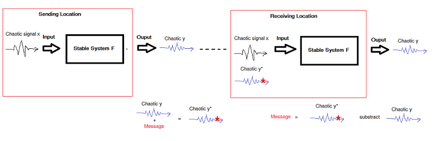
Referring to the figure below, at the sending location chaotic signal x is generated and
fed into a stable system F to produce the output as another chaotic signal y. Message
encryption occurs when the message is mixed with the chaotic signal y and the result is
the message-carrying signal y* that has a chaotic behaviour. Next step is to transmit
two signals to the receiving location. One is the original chaotic signal x and the
other is the message-carrying chaotic signal y*. At the sending location only chaotic
signal x is fed into another stable system F which is identical to the stable system F
at the sending location. Therefore, the output will be the chaotic signal y, which is
the same output produced by the corresponding stable system F at the sending location.
Finally, the original message can be recovered by subtracting chaotic signal y from the
message-carrying chaotic signal y* at the receiving location. [3]
Interested Concentration
A Lorenz system is a system of ordinary differential equations with chaotic solutions for
certain parameter values and initial conditions. When plotted, the system resembles a
butterfly, hence chaos theory is often time called the Butterfly Effect. A simple
analogy is the following: a flap of a butterfly in Mexico can cause a tornado in Texas.
The notion is that a slight change in the current state could potentially cause a
drastic change in the long-term effect, thus the validity of the starting points is
highly sensitive.
\begin{eqnarray} \frac{dx}{dt}&=& \sigma (y-x)\\ \frac{dy}{dt}&=&
x(\rho-z)-y\\ \frac{dz}{dt}&=& xy-\beta z \end{eqnarray}
In Lorenz system, $x$, $y$, and $z$ are the system state, $t$ is time, $\sigma$, $\rho$,
and $\beta$ are the system parameters. The constants $\rho$, $\beta$, and $\sigma$
determine the behavior of the system. Lorenz defines a deterministic sequence as one in
which only one thing can happen next from an existing event. Furthermore, deterministic
chaos is something that looks random, but is still deterministic. For the purpose of
this page, we will use the canonical parameters $\rho=10$, $\beta=\frac{8}{3}$, and
$\sigma=28$.
Mathematics and Procedure
Any $n^{th}$ order linear ordinary differential equation can be expressed in the form of
a system of first order linear ODEs. Numerical approximation is applied to ascertain
values that may otherwise be impossible to solve through traditional methods. One
popular family of numerical methods is the Runge Kutta which carries a better
computational accuracy than the other methods [4]. Runge Kutta method consists of a
number of numerical methods that can provide different levels of accuracy. Runge Kutta
Fourth Order is one of the Runge Kutta methods and was introduced in the class.
Therefore, the goal of this study is to introduce a new Runge Kutta method called
Adaptive Runge Kutta method that is hypothetically capable of providing a better
accuracy and efficiency than Runge Kutta Fourth Order method. The procedure in this
study is to solve the Lorenz attractor by using both Adaptive Runge Kutta and RK4
methods and compare the results. The motivation for comparing the two methods is that
the efficiency gained in adaptive RK can be hundred times or more compared to RK4 [5].
Nomenclature
$h$
Time step
$\rho, \beta, \sigma$
Parameters of the Lorenz Attractor
$x_0, y_0, z_0$
Initial Conditions, highly sensitive to the system
$k_i$
Increment based on the slope
Runge Kutta Fourth Order
As presented in the class, Runge Kutta Fourth Order or RK4 is one amongst a family of
numerical methods developed by two German Mathematicians C. Runge and M.W. Kutta that
are cable of approximating the solutions to ordinary differential equations by
discretizing both spatial and temporal domains. Runge Kutta methods can also be
extended to solve a system of initial value problems (IVPs) which is the case for the
Lorenz Attractor. RK4 requires four function evaluations as presented in equation 4 to
8 and it has an error in the order of $O(h^4)$ [6].
$$ dx(t) = f(x,t) \quad x(0)= x_0
= a$$ $$k_1 = hf(t_i,x_i)$$ $$k_2 = hf(t_i+\frac{1}{2}h,x_i+\frac{1}{2}k_1)$$ $$k_3 =
hf(t_i+\frac{1}{2}h,x_i+\frac{1}{2}k_2)$$ $$k_4 = hf(t_i+h,x_i+k_3)$$ $$x_{i+1} =
x_i+\frac{1}{6}(k_1+2k_2+2k_3+k_4)$$ where $h$ is the size step and $t_i=t_0+ih$
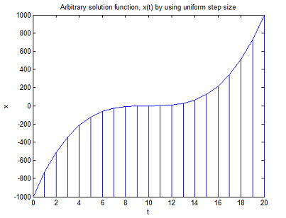
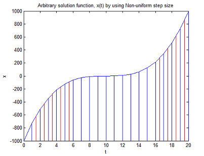
Adaptive Runge Kutta
Adaptive Runge Kutta method is the extension of RK4 method in that RK4 uses a uniform
time step size throughout the entire domain (Figure 2.a) while Adaptive RungeKutta
method uses non-uniform time step size by employing the step size control method in
order to obtain an estimate within a prescribed tolerance $\epsilon$ and with a minimum
computational effort. The purpose of adapting the step size is to use smaller steps with
steep slope regions of the solution curve and to use larger steps with shallow slope
regions of the solution curve in order to obtain an estimate within $\epsilon$
In order to adapt the step size, expected error estimate is needed to compare to the
prescribed tolerance, $\epsilon$. If the expected error is smaller or equal to the
tolerance, the current step size shall be used for the next step otherwise a new step
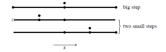
size is to be computed based on the estimate error. There are two common methods in
estimating the expected error. The first method, called step doubling, is to take each
step twice using step sizes $h$ as full step and $h/2$ as two small steps. The expected
error is calculated as the difference between the two results. The second method is to
use higher-lower order method in which the idea is to calculate the error as the
difference between results from two order methods, say 4th and 5th, and adapt a unique
step size for the next time step throughout.The adaptive Runge Kutta method conducted
in this study is the Runge Kutta Fehlberg method, also known as Embedded Runge Kutta
Formulas (RK45) [5].
Runge Kutta Fehlberg Method (RK45) was developed by a German mathematician Erwin
Fehlberg in 1969 with error in order of $O(h^5)$. RK45 requires six function
evaluations. A combination of these functions provides the calculation of the next step
based on RK4, $x_{i+1}^{RK4}$, (eq.15) and a different combination of these functions
provides the calculation of the next step based on RK5, $x_{i+1}^{RK5}$
If $R <=\epsilon$ keep $x$ as the current step solution and move to the next step with
step size $\delta h$.
If $R>\epsilon$ recalculate the current step with step size $\delta h$.
Step-doubling as a means for adaptive stepsize control in fourth-order Runge-Kutta.
Points where the derivative is evaluated are shown as filled circles. The open circle
represents the same derivatives as the filled circle immediately above it, so the total
number of evaluations is 11 per two steps. Comparing the accuracy of the big step with
the two small steps gives a criterion for adjusting the stepsize on the next step, or
for rejecting the current step as inaccurate [5].
Result and discussion
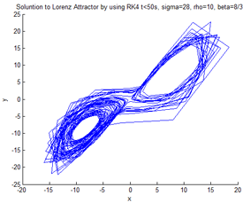
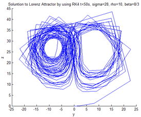
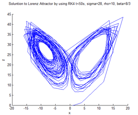
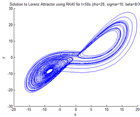
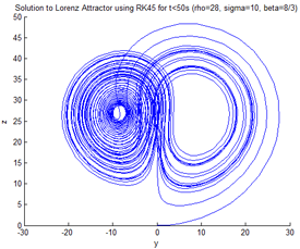
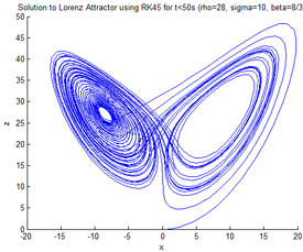
The solutions to Lorenz Attractor found using both methods are presented in Figure 4.
These results are projected onto three principal planes xy, yz and xz for the purpose of
comparison. It can be observed that in general the plots of solution after a given time,
t, from RK45 are smoother than those from RK4. This indicates that RK45 is capable in
providing a more accurate result than RK4.
The top row was plotted using RK4 and the bottom row RK45. It is
clear that RK45 produces smoother plots and one explanation has to do with a larger
discretization of the time interval. Whereas RK4 uses a for loop algorithm since the
time step is constant for every iteration, RK45 uses a while loop because the algorithm
readjusts the time step to minimize the error difference within a tolerance.
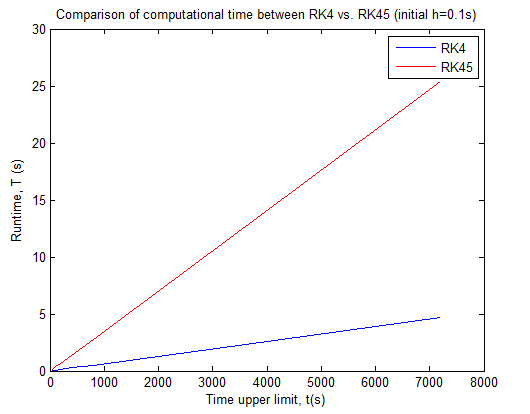
Above is a plot of comparison of computational time between RK4 and RK45 for solving
Lorenz Attractor. Initial step size used is h=0.1s. Although, RK45 provides a more
accurate estimate of the solution within a prescribed tolerance however it is more
computationally expensive. Figure 6 shows the plot of comparison of the computational
time between RK4 and RK45 for solving the Lorenz Attractor. Both methods start with the
initial time step $h=0.1 seconds$. Horizontal axis is the time upper limit, t, in
seconds; while the vertical axis is the runtime in seconds for each time upper limit. In
light of the accuracy in data taking, for each time upper limit, the runtime was taken
for three test runs and the average of these three runs are used to plot the
relationship between time upper limit versus runtime. The graphs obtained from both
methods are approximately linear line. By using the linear regression in MALAB, the
slope of RK4 and RK45 are 0.00065 and 0.0035, respectively. This indicates that as time
progresses the runtime for solving the Lorenz Attractor increases by a factor of 0.00065
and 0.0035 for using RK4 and RK45, respectively.
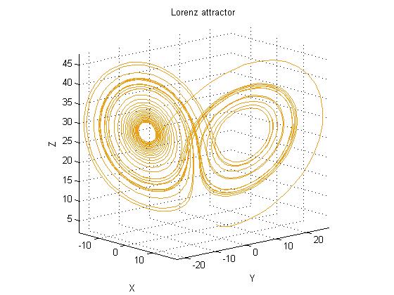
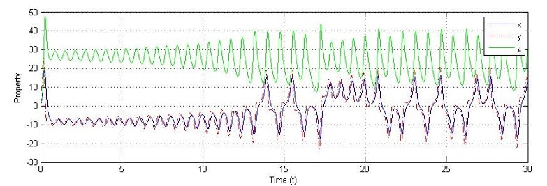
Lorenz Attractor with $\rho=28 \; \sigma=10 \; \beta=8/3$
The time spectrum on Figure 7 suggests that the system is always fluctuating and no
equilibrium (dynamic or static) is ever reached. Moreover, for a deterministic system,
one would expect Figure 6 to have a constant fluctuation (much like a sine wave or
horizontal line), but it is clear that the attractor begins to exhibit a chaotic
behavior after $t=13$. This is essentially the main idea of chaos theory - that
deterministic system never achieves a steady state and trajectory never coincides with
any other (See Figure 6). Using both Runge Kutta methods, one thing is certain, it
doesn't matter how close two different initial conditions are, their trajectories will
eventually diverge.
Conclusion
The fact that the Lorenz attractor is sensitive to its starting point to a plausible
extent suggests that Weather is usually predictable only about a week ahead [11]. Long
term prediction cannot be made due to the system’s chaotic behavior after some t time. A
future study can be examined in the context of random data versus chaotic data. This
page solely seeks a comparison between the two Runge Kutta methods as a numerical
approximation to study the theory, but real life application calls for unwanted and
corrupting noises. Theoretically, even when the system is deterministic, the real time
series will consist of a few stochastic data, therefore one should be careful when
defining the error as the difference between the time evolution of the ’test’ state and
the time evolution of the nearby state. Finally, it is without a doubt that studying
chaos theory will provide mankind better control of the predictibility of standard
living, but we are far from comprehending its chaotic behavior. It is difficult to even
a simplify a gaseous system in a small domain, let alone simulate the weather by
breaking the atmosphere into many millions of interactive systems and predict the
weather for next month since we don’t know the initial conditions at time t=0 very
accurately.
References
Danforth, Christopher M. Chaos in an Atmosphere Hanging on a Wall,
Mathematics of Planet Earth, 2013.
Fractal Foundation, What is Chaos Theory, Fractals are Smart: Science, Math
and Art! http://fractalfoundation.org.
George, Yurkon T. (1997). Introduction to Chaos and It's Real World Applications.
http://www.csuohio.edu/sciences/dept/physics/physicsweb/kaufman/yurkon/chaos.html.
Camhdag, Ezel. Runge Kutta Methods. Cankaya University, January 27, 2009.
Press, W. H. (1996). Chapter 16. Integration of Ordinary Differential Equations.
Numerical recipes in fortran 77: the art of scientific computing (2nd ed.,
pp. 701-744). Cambridge [England: Cambridge University Press.
Press, William H. , Teukolsky, Saul A. , Vetterling, William T, and Flannery, Brian
P. Numerical Recipes in C, Second Edition, Cambridge University Press 1992.
Bradley, Larry. Chaos and Fractals, 2010
http://www.stsci.edu/~lbradley/seminar/references.html.
Kellert, Stephen H. In the Wake of Chaos: Unpredictable Order in Dynamical
Systems, University of Chicago Press 1993. p. 32.
Sparrow, Colin. The Lorenz Equations: Bifurcations, Chaos, and Strange
Attractors, Springer 1982.
Hilborn, Robert C. Chaos and Nonlinear Dynamics: An Introduction for Scientists
and Engineers (second ed.). Oxford University Press 2010.
Watts, Robert G. (2007). Global Warming and the Future of the Earth. Morgan and
Claypool. p. 17.
Master of Science in Computational Mechanics at Carnegie Mellon University,
May 2014 Bachelor of Science in Structural Engineering with Minor in Mathematics at the
University of California, San Diego, June 2011
Objective
Seeking a full time position to gain hands-on experience by applying knowledge
to real-life engineering applications (specifically in the field of software design and
computational analysis) and acquire managerial skills in an industrial environment.
Skills/ Qualifications
Familiar in SAP2000, Visual Basic (VB.NET) & Visual Basic for Application (VBA),
C/C++/C#, Java, SharePoint
Proficient in Autodesk Products (AutoCad, Inventor), Wordpress, JavaScript &
JQuery
Other (Engineer-in-Training Certificate, fluency in English and Vietnamese)
Relevant College Courses and Projects
Finite Element
Development of mass and stiffness matrices based upon virtual work for static and dynamic
problems. Solidworks was used for computational analysis in draft and high quality
finite elements.
Foundation Design and Earthquake Engineering
Soil examination and it-situ testing for foundation analysis. Topics on shallow
foundation and bearing capacity were discussed. Seismic detailing involved elastic and
inelastic response spectra for a modal analysis of ground motion.
Internship
UCSD Pacific Rim Experience for Undergraduate (PRIME) - Research
Internship at the University of Auckland, New Zealand (Summer 2010)
Assisted in the construction of steel frame and prepared bracket materials. Identified
loading cell sensor locations of unreinforced masonry structures for testing of New
Zealand existing buildings. Recorded data of timber-floor diaphragm for simulation to be
stored and managed in NeesCentral data repository.
City of Los Angeles – Office of Public Works, Wastewater Conveyance Engineering Division
(Fall 2012)
Identified and surveyed Secondary Sewer Renewal Program (SSRP) daily reports to tabulate
equipment usage, manpower, and pipe liner installation through an internal database.
Prepared a technical paper (co-author) that demonstrated the benefits of trenchless
methods/technologies to reduce carbon footprint – (2013) Trenchless in Los Angeles,
Secondary Sewer Rehabilitation Carbon Footprint. North American Society for Trenchless
Technology 2013 Conference - No-Dig Show (TM1-T1-01). Retrieved from http://nastt.org
Employment History
Michael Baker International Civil Associate II / Software Developer Primarily responsible for generating
algorithms in C++/C# for AASHTOWARE Bridge Design and Bridge Rating (BrDR) software in
.NET framework. Primary developer for an in-house project management tool that utilizes
the MVVM pattern and Entity framework. Serve as the leader and mentor a UI team of 8
members. Supervise members’ daily tasks. Design graphical user interfaces using WPF and
XAML in accordance to Microsoft’s guidelines. Write programs for bridge design and
evaluation in LRFD, ASR, LFR and LRFR specifications. Support bridge engineering and
update software system based on latest specifications. Populate engineering reports in
XML and XSLT languages Support and update software's website in SharePoint. Conduct and
approve code reviews on front end related development. Design and maintain model domains
for data access.
Pittsburgh, PA June 2014 – Current
University of Pittsburgh Adjunct Math Instructor Taught and developed the subject curriculum. Prepared
and provided students with course outlines and syllabus. Assessed student performance
and maintain grade records. Created an effective learning environment through the use of
a variety of instructional methods. Prepared lesson plans and covered conceptual topics
that meet the department’s requirements. Courses vary from applied calculus to linear
algebra and differential equations.
Pittsburgh, PA June 2015 – May 2017
Janmar Lighting Solidworks Drafter / Production Artist Assist the senior engineer in drafting
of lighting components in Solidworks and manage company’s website with technical
support. Responsible for the production of engineering spec sheets and BOM for
manufacturing and tailor designs according to clients’ demands. Write programs in VBA
for daily purposes in Microsoft Suite.
Covina, CA December 2012 - June 2013
Can Academy Math Teacher Teach middle and high school students mathematics from algebra
to calculus in a classroom setting. Monitor students’ progress and prepare them for the
California STAR testing
West Covina, CA September 2012 - June 2013
iD Tech Camp Technology Instructor Prepared lesson plans and taught students (ages 7-17)
various classes from digital photography to video game design and programming (in C++
and Java) at UCI and UCSD. Conducted activities and promoted friendly atmosphere for
large groups of children.
Irvine & San Diego, CA Summer 2012 & 2013
Melrose Creations Inc. Graphic Design Intern Designed website layout, created sale sheets and other
printed material for promotional sales, and redesigned company’s website.
City of Industry, CA Jan 2012 – June 2012
Tutor Doctor | Club Z! Language Art and Math Tutor Tutor students from HS to college in various
subject including mathematics (algebra to advanced calculus).
San Gabriel River Valley, CA Jan 2012 – June 2012
Rady School of Management HelpDesk Technician/ Video Recorder and Editor Served customers with computer
technical issues, recorded classroom lecture sessions, edited and rendered content to
RADAR.
University of California, San Diego Oct 2008 – August 2011
UCSD Transportation Shuttle Driver Drove the shuttle bus, managed customer service, and trained
prospective drivers.
University of California, San Diego June 2009 – June 2011
Study ABroad Experience
UCSD Global Seminar- Mathematical Beauty
in Rome (2008)
Studied architectural analysis and structural concepts of Roman classical buildings in
Rome, Italy.
Free University of Berlin, Germany – Architecture in Berlin from the 19th Century to Today
(2011)
Examined the foundation and main façade of famous buildings in Berlin from Classical
order to the International Style.
Leadership
Muir College House Officer UCSD Strides Running Club (Vice President)
Sep 2009 – June 2010 June 2009 – June 2011
Favorite Quote
A journey of a thousand miles begin with the first step - Laozi
Experience is not what happens to a man, it's what he does with what happens to him -
Aldous Huxley
Friends are like a bra, close to your heart and there for support - Ethan Uong
I am the master of my fate, the captain of my soul. - William Ernest Henley
The two most important days of your life are the first day you were born, and the day you
find out why - Mark Twain
Live as if you were to die tomorrow. Learn as if you were to live forever -
Ghandi
It’s better to look back on life and say, “I can’t believe I did that,” than to look back and
say, “I wish I did that.” - Marc Chernoff
To the world you may be one person, but to one person you may be his world - Dr.
Seuss
Falling down is part of life, getting back up is living - Jose Harris
Don’t forget who you are, you’re a nobody if you don’t know where you come from- Ethan
Uong
Multimedia Fusion
** I made the following two Flash games when I taught video-game design at iD Tech.
If you have it, you want to share it. If you share it,
you don't have it. What is it?
A secret!
What gets whiter the dirtier that it gets?
A chalkboard!
What goes on four legs in the morning, on two legs at
noon, and on three legs in the evening?
A man, who crawls on all fours as a baby, walks on two legs as an adult, and walks with a
cane in old age!
Who is the best looking engineer in the world?
Da Ethanator (no-brainer)!!
You are stuck in a big steel box with only a locked
door and a piano, how do you escape?
Play a key on the piano and use the key to open the door!
4 men in a boat on the lake, boat turned over and they
all sink to the bottom of the lake, yet not a single man got wet! Why?
Because they were all married and not single!
He has married many women, but has never been married.
Who is he?
A preacher!
The more it dries, the wetter it gets. What is it?
A towel!
Imagine you are in a sealed room with absolutely
nothing, how do you get out?
Stop imagining!!
What is the end of everything?
The letter g (of everything)!
There is a room with just a mirror and a table. How
do you get out?
You look in the mirror and see what you saw, you take the saw and saw the table in half, 2
halves make a whole and you climb out the hole!
I am a rock group that has 4 members, all of whom are
dead, one of which was assassinated. Who am I?
Mount Rushmore! Get it!? Rock group, 4 members = presidents...
What is close to your heart and there for support?
A bra!
You're stuck a sealed room with nothing but a
baseball and baseball bat, how do you get out?
You serve the ball to yourself and miss, strike 1, strike 2, strike 3, you're out!
I work on a horse racetrack and have a meeting that
lasts a week. I leave on Friday but return on Monday, how is this possible?
I went to the meeting on a horse named Friday.
A series of riddles
An airplane has 500 bricks, you throw one off,
how many are left?
500 - 1 = 499 bricks left
What are the three steps to put an elephant in
a refrigerator?
Open the refrigerator, put the elephant in, close the door
What are the four steps to pur a deer in the
refrigerator
Open the refrigerator, take the elephant out, put the deer in, close the door
Lion King is having a party, all animals are
there except one, which one is it?
The deer, he's still in the fridge
Grandma crosses a swamp with no injury, how is
that?
Alligators and crocodiles are at the party
Once Grandma gets to the other side, she dies.
Why?
She is hit by the brick you threw off!
Get in touch with me
Please let me know your suggestions, comments or even concerns by filling out the form
below. Please keep in mind that while I do read all emails that come in, I am not able to
respond to all of them.
School, Piano, Reading, Engineering, Traveling, Gym, Photography, Tennis, Poker
Ethan Thomas Uong (born January 18) is an Asian-American
engineer and residing in Los Angeles, CA. Uong graduated from the University of California, San
Diego with a degree in Structural Engineering (emphasis on geotechnical design and computational
analysis) and Carnegie Mellon in M.S Computational Mechanics. He is the recipient of the
American Society of Civil Engineers award and scholar of the Leo Politi Foundation. Currently,
he works for Baker International as a software developer for bridge engineering in AASHTO
specifications. Uong is perhaps best known for his natural curiosity, willingness and dedication
for learning, and pragmatic approach on solving problems.
When he was in college, Uong had three opportunities to study abroad including an internship in
New Zealand. It was through these experiences that he was able to see life in a more optimistic
perspective. With his camera, Uong has captured many famous landmarks including some classical
and modern Wonders of the World such as the Roman Colosseum and Milford Sound. It is his dream
to capture the perfect picture in each continent.
Early Life and Education
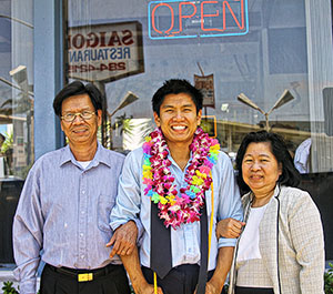
Uong and his parents at his UCSD
graduation
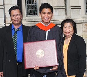
Uong's CMU graduation - one of
the proudest moments of his life
Born to native parents from Ho Chi Minh City in Vietnam, Uong is the youngest of three siblings.
With hardworking parents, the Uong family immigrated to the United States with high hopes for
their future. As a young child, Uong had little interest for learning and associated more to
music and athletics. Eventually learning the importance of education and with inspiration from
his parents, Uong persevered throughout the four years he spent in college majoring in
Structural Engineering while getting a minor in Mathematics. Even as a working student, Uong
consistently attained high marks in his classes and continued to maintain an active and healthy
lifestyle by joining a running club and serving as its vice president.
At a young age, Uong had a candid characteristic to break things apart and put them back together
and this attitude brought out this true passion in Computational Mechanics where he is able to
wander endlessly in the world of mathematics and science. The very thing (airplane) that took
him to the land of opportunity is a work of technology and innovation, and he is determined to
make a difference in the tech industry. Uong envisions computing and analyzing structures of all
kind in the nearby future to develop a systematic and economical approach to engineering
problems.
Travel
With a great sense for cultural awareness, Uong has visited many countries throughout his time in
college including Rome, New Zealand, and Germany. He frequently traveled across the world as a
college student gathering an abundant amount of experience for each of the places he visited.
With no hesitation and fear, he stepped onto new territories and allowed his experiences to
diversify his view of the world. Uong continues to believe that a worldly experience can lead to
success. For Uong, knowledge is power and with power, comes the ability to positively influence
people’s lives. Each time he traveld abroad, he obtained a vast knowledge of their culture and
gained a better appreciation of his own.
Personal Life
Uong is considered a world traveler for having been to over 12+ countries. He loves diversity and
believes it to be the key to success and acceptance. In his spare time, Uong likes to play his
Rodriguez flamenco guitar, pick up a computer language, or go for a jog. Uong's biggest dream is
to be a well-respected and ethical engineer to contribute society's needs. His next big move in
life is earning an MBA to advance his career and saving money to travel to the Mediterranean! :)


 - Füssen, Germany")


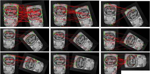
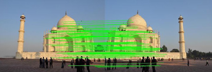 Suppose $p \propto Hq$ where
$p=[x',y',z']^T$ and $q=[x,y,z]^T$ for $p,q$ respectively, then $$ \left \{
\begin{array}{c} x'\\y'\\z' \end{array} \right\} \sim \left[ \begin{array}{ccc}
h_{11} & h_{12} & h_{13} \\ h_{21} & h_{22} & h_{23} \\ h_{31} & h_{32} & h_{33}
\end{array} \right] \left \{ \begin{array}{c} x\\y\\z \end{array} \right\}
\rightarrow \left \{ \begin{array}{c}
x'=\frac{h_{11}x+h_{12}y+h_{13}}{h_{31}x+h_{32}y+h_{33}}\\\\y'=\frac{h_{21}x+h_{22}y+h_{23}}{h_{31}x+h_{32}y+h_{33}}
\end{array} \right. $$\\ If we multiply both sides by the denominator and arrange,
we get $$ \left \{ \begin{array}{c} x'=h_{11}x+h_{12}y+h_{13}-h_{31}xx'-h_{32}yx'-x'
\\ y'=h_{21}x+h_{22}y+h_{23}-h_{31}xy'-h_{32}yy'-y' \end{array} \right. $$ To
minimize the homogenous linear least squares system we seek $arg \; min ||Ah|| = arg
\; min \;h^TA^TAh = \lambda_{min}$ If we decompose A using SVD method, the planar
homography is precisely the last column of D corresponding to the smallest
eigenvalue. Furthermore, if the eigenvalues are zero, h is exactly determined and
fits all the points perfect. If the values are positive, the system is
overdetermined and a residual will exist.
Suppose $p \propto Hq$ where
$p=[x',y',z']^T$ and $q=[x,y,z]^T$ for $p,q$ respectively, then $$ \left \{
\begin{array}{c} x'\\y'\\z' \end{array} \right\} \sim \left[ \begin{array}{ccc}
h_{11} & h_{12} & h_{13} \\ h_{21} & h_{22} & h_{23} \\ h_{31} & h_{32} & h_{33}
\end{array} \right] \left \{ \begin{array}{c} x\\y\\z \end{array} \right\}
\rightarrow \left \{ \begin{array}{c}
x'=\frac{h_{11}x+h_{12}y+h_{13}}{h_{31}x+h_{32}y+h_{33}}\\\\y'=\frac{h_{21}x+h_{22}y+h_{23}}{h_{31}x+h_{32}y+h_{33}}
\end{array} \right. $$\\ If we multiply both sides by the denominator and arrange,
we get $$ \left \{ \begin{array}{c} x'=h_{11}x+h_{12}y+h_{13}-h_{31}xx'-h_{32}yx'-x'
\\ y'=h_{21}x+h_{22}y+h_{23}-h_{31}xy'-h_{32}yy'-y' \end{array} \right. $$ To
minimize the homogenous linear least squares system we seek $arg \; min ||Ah|| = arg
\; min \;h^TA^TAh = \lambda_{min}$ If we decompose A using SVD method, the planar
homography is precisely the last column of D corresponding to the smallest
eigenvalue. Furthermore, if the eigenvalues are zero, h is exactly determined and
fits all the points perfect. If the values are positive, the system is
overdetermined and a residual will exist.

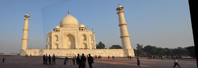
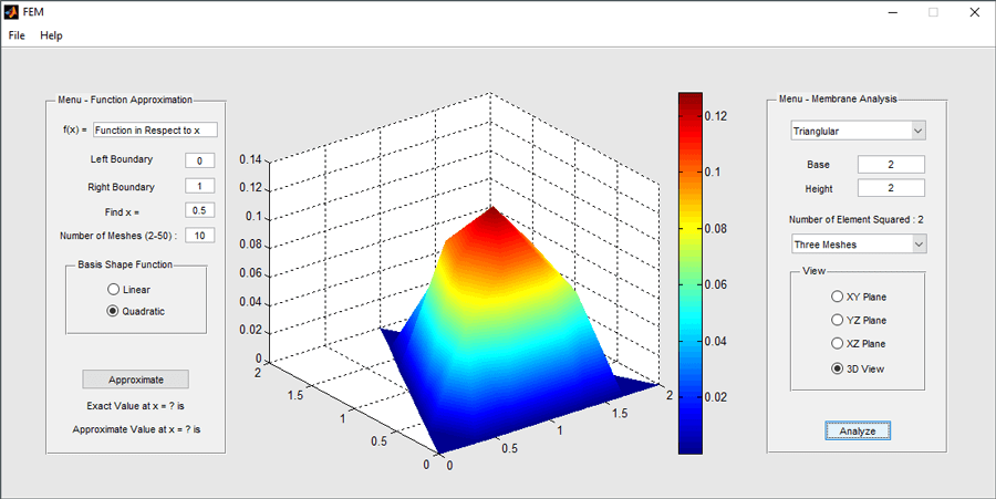


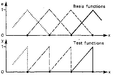
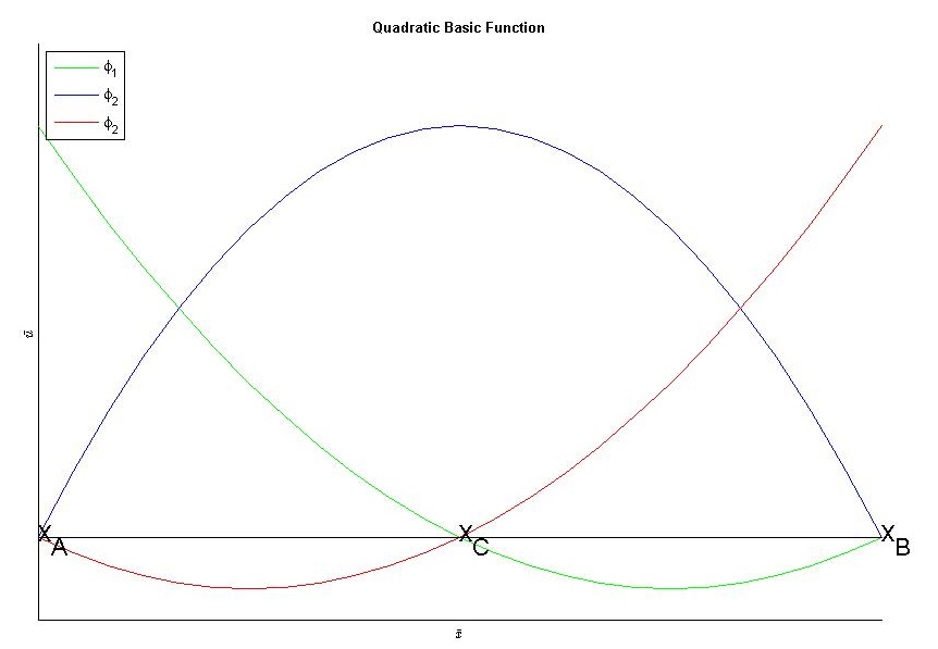
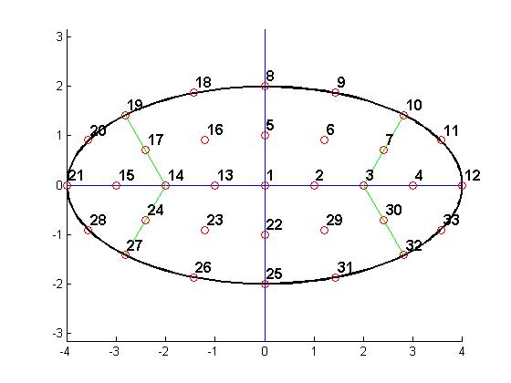
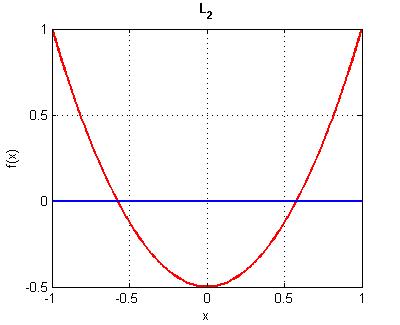
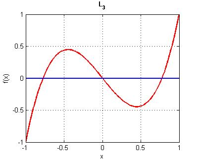
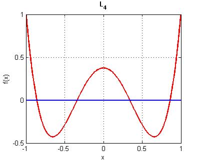
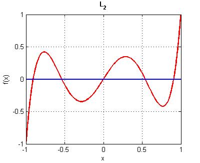
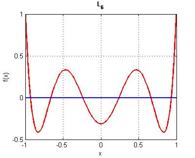
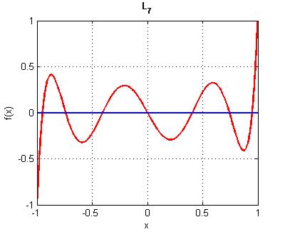
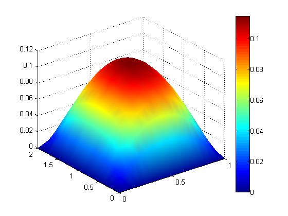
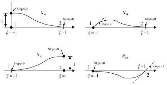 \begin{eqnarray} N_1(\xi)=\frac{1}{4}(1-\xi)^2(2+\xi)\\
N_2(\xi)=\frac{h}{8}(1-\xi)^2(1+\xi)\\ N_3(\xi)=\frac{1}{4}(1+\xi)^2(2+\xi)\\
N_4(\xi)=\frac{h}{8}(1+\xi)^2(\xi-1)\\ \end{eqnarray} Local Stiffness Matrix
$$K_{ij}=\int_eEI\frac{d^2N_i(x)}{dx^2} \frac{d^2N_j(x)}{dx^2}dx=\int_{-1}^1
EI\frac{d^2N_i(x)}{dx^2} \frac{d^2N_j(x)}{dx^2}\frac{1}{2}h d\xi$$ For a generic case
with both free nodes, the matrix becomes \[ K^e = \frac{EI}{h^3}\left[
\begin{array}{cccc} 12 & 6h & -12 & 6h \\ 6h & 4h^2 & -6h & 2h^2 \\ -12 & -6h & 12 & -6h
\\ 6h & 2h^2 & -6h & 4h^2 \end{array} \right]\] Local Force Vector $$f_i^{(e)}=\int_e
q(x)N_i(x)dx=\int_{-1}^1 q(x)N_i(x)\frac{1}{2}h d\xi$$ For uniform load $q_0$
$$f^{(e)}=\frac{q_0h_e}{12} \left\{ \begin{array}{c} 6\\ h_e \\ 6 \\ -h_e \end{array}
\right\} $$ System array is defined with dimensions $n\;x\;m$ where $n$ is 4 (the number
of degree of freedom per element) and $m$ is 3 (the number of elements).
\begin{eqnarray} N_1(\xi)=\frac{1}{4}(1-\xi)^2(2+\xi)\\
N_2(\xi)=\frac{h}{8}(1-\xi)^2(1+\xi)\\ N_3(\xi)=\frac{1}{4}(1+\xi)^2(2+\xi)\\
N_4(\xi)=\frac{h}{8}(1+\xi)^2(\xi-1)\\ \end{eqnarray} Local Stiffness Matrix
$$K_{ij}=\int_eEI\frac{d^2N_i(x)}{dx^2} \frac{d^2N_j(x)}{dx^2}dx=\int_{-1}^1
EI\frac{d^2N_i(x)}{dx^2} \frac{d^2N_j(x)}{dx^2}\frac{1}{2}h d\xi$$ For a generic case
with both free nodes, the matrix becomes \[ K^e = \frac{EI}{h^3}\left[
\begin{array}{cccc} 12 & 6h & -12 & 6h \\ 6h & 4h^2 & -6h & 2h^2 \\ -12 & -6h & 12 & -6h
\\ 6h & 2h^2 & -6h & 4h^2 \end{array} \right]\] Local Force Vector $$f_i^{(e)}=\int_e
q(x)N_i(x)dx=\int_{-1}^1 q(x)N_i(x)\frac{1}{2}h d\xi$$ For uniform load $q_0$
$$f^{(e)}=\frac{q_0h_e}{12} \left\{ \begin{array}{c} 6\\ h_e \\ 6 \\ -h_e \end{array}
\right\} $$ System array is defined with dimensions $n\;x\;m$ where $n$ is 4 (the number
of degree of freedom per element) and $m$ is 3 (the number of elements).